Particle Tracking Challenge

Conditions of usage

• Challenge image data for virus scenario
• Challenge image data for vesicle scenario
• Challenge image data for receptor scenario
• Challenge image data for microtubule scenario
• Challenge ground truth for all scenarios

As announced, the particle tracking challenge are based on computer generated data only, in order to allow accurate, quantitative performance evaluation of all methods under controlled conditions, with hard and objective ground truth. This requires simulation of particle imaging to a hopefully good level of realism. In practice, there are many variables (microscope settings, particle properties, image parameters) that could be varied, and for which the performance of tracking methods could be evaluated. Needless to say, the space spanned by these variables is very high-dimensional, and would require a very large set of sample image data to explore. To make the challenge feasible, we focus on three key aspects affecting the performance of particle tracking algorithms: (1) different particle imaging scenarios, (2) different signal-to-noise ratios (SNR) of the data, and (3) different levels of particle density.

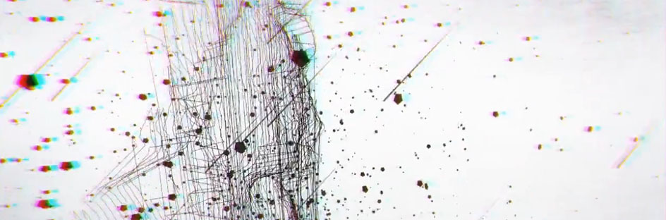
Four different scenarios are selected for the challenge, mimicking real image data of moving viruses, vesicles, receptors, and microtubule tips. For each of these scenarios, image data were generated at four different SNR levels (Poisson noise was used as this is the limiting case in microscopy), and of three density levels. As indicated in several papers in the literature, SNR=4 is a critical level at which methods may start to break down. We selected this level, and added one higher level (SNR=7), one lower level (SNR=2), and one very low level (SNR=1). Note that a given SNR indicates the maximum SNR in that data (it drops as particles move out of focus). As for density, we defined three categories, depending on the scenario: low density (on the order of 50-100 particles), mid density (100-500 particles), and high density (on the order of 1000 particles or even more). All particles are subresolution in size. Their exact size (relative to pixel size) and numbers, their dynamics, as well as their start and end frames (in time), are slightly randomized to mimic reality, in which case these values are not known exactly, either.

A brief description of the image data for the four scenarios:

Viruses

• Particle shape: spherical
• Dynamics: same direction, switch between brownian and linear
• PSF: Airy disk profile
• Densities {low, mid, high}: {100, 500, 1000}
• Dimensionality: 3D+time
• z-step: 300nm
• Image size: 512x512 pixels
• Image depth: 10 slices
• Image length: 100 frames

Download the images and ground truth tracks from this scenario here.

Vesicles

• Particle shape: spherical
• Dynamics: brownian, any direction
• PSF: Airy disk profile
• Densities {low, mid, high}: {100, 500, 1000}
• Dimensionality: 2D+time
• Image size: 512x512 pixels
• Image length: 100 frames

Download the images and ground truth tracks from this scenario here.

Receptors

• Particle shape: spherical
• Dynamics: tethered motion, switching, any direction
• PSF: Airy disk profile
• Densities {low, mid, high}: {100, 500, 1000}
• Dimensionality: 2D+time
• Image size: 512x512 pixels
• Image length: 100 frames

Download the images and ground truth tracks from this scenario here.

Microtubules

• Particle shape: slightly elongated (tips)
• Dynamics: nearly constant velocity model
• PSF: Gaussian intensity profile
• Densities {low, mid, high}: {60, 400, 700}
• Dimensionality: 2D+time
• Image size: 512x512 pixels
• Image length: 100 frames

Download the images and ground truth tracks from this scenario here.

The ground truth particle positions and tracks in the training image data are provided in XML format as in the example below. Each training set (that is, a given scenario, SNR level, and particle density level) has a separate XML file associated with it. The file specifies (in XML terms) the position (x,y,z) of each particle at each relevant time point (t). The spatial coordinates (x,y,z) of particle positions can be specified with floating-point precision. These coordinates run from 0 (center position of the first pixel position in any dimension) to N-1 (center position of the last pixel position in any dimension). The temporal coordinate (t) is an integer index, which may run from 0 (first frame) to N-1 (last frame), but only the relevant time points need to be specified.

NOTES:

• Please respect the case (lower, upper, proper) of all tags as indicated in the above example.
• The 'snr' keyword and value must be written in lowercase. Valid values are: 1, 2, 4, or 7.
• The 'density' keyword and value must be written in lowercase. Valid values are: low, mid, or high.
• The 'scenario' keyword and value must be written in lowercase. Valid values are: virus, vesicle, microtubule, or receptor.
• The 'detection', 't', 'x', 'y', 'z' keywords must be written in lowercase.
• The decimal separator is '.'

The above XML format is the format that is used in the final evaluation of the challenge. Participants are requested to add some code to their algorithms that exports the tracking results to a file in this format. The evaluation software described below also uses this format and can be used by the participants to pre-test the performance of their algorithms during the training phase.

All softwares are now available directly in the imaging software Icy. Simply type their name in the search bar of Icy and click on the result. Selected plugin are automaticaly installed. The source code is included in jar files, available in Icy or directly from the Icy website. The following software list display the plugins and their usage:

1. Tracking Performance Measures: Computes the score of a set of track vs the ground truth.
2. ISBI Challenge Track Generator: Generates tracks for benchmark, providing access to a large number of generation parameters.
3. ISBI Challenge tracking benchmark generator: Compute a whole benchmark with all scenarios.
4. ISBI Challenge Tracks Importer: TrackProcessor for the TrackManager plugin that allows importing/exporting tracks.
5. ISBI Tracking Challenge Batch Scoring: Automation of scoring for large dataset. Based on Tracking performance measures plugin.

To quantitatively evaluate tracking performance, we defined a set of performance measures, as detailed in this technical note (PDF file). These are the measures that are used in the final evaluation and that are also implemented in the evaluation software tools described below. In summary, the performance evaluation procedure consists of two steps:

During the tracking challenge, two software platforms are made available to the participants for evaluating their own tracking results in the training phase. Both are open-source platforms based on Java. The first is a stand-alone application and the second one is a plugin called Tracking Performance Measures that can be directly downloaded from the imaging software Icy. The main difference between the two platforms is that Icy is shipping visualization tools for tracking results. In the case of the stand-alone application, one needs to use a third-party software for visualizing tracks.

One has first to download the evaluation software which includes a manual describing its use and its source code. The application can be launched using the following command:

java -jar trackingPerformanceEvaluation.jar [-OPTIONS]

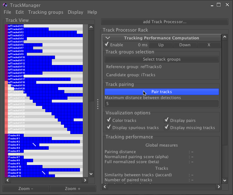
where [-OPTIONS] stands for input options that are described in the manual of the application. If no input option is specified, the following graphical user interface is displayed:

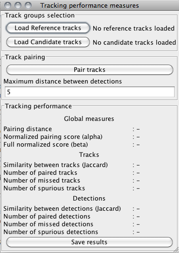
The XML files containing tracks information can be specified in the Track groups selection box. In the Track pairing box, the distance field is the gate ε that is used for measuring distances between particle positions, as described in the technical note mentioned above. Once the Pair tracks button is clicked, the optimal pairing is computed and the tracking performance criteria are automatically displayed in the box Tracking performance. The results can be exported to a text file by clicking Save results.

The performance evaluation software can also be used in command-line mode. One has then to specify the track files as the input arguments of the application. For instance, entering the command:

java -jar trackingPerformanceEvaluation.jar -r groundTruthTracks.xml -c builtTracks.xml

yields the computation and display of the tracking performance measures for ground truth file groundTruthTracks.xml and candidate tracks file builtTracks.xml.

The stand-alone application does not feature visualization tools for tracks. A solution for visualizing tracks is the MTrackJ plugin for the image analysis software ImageJ. Tracks stored in XML files in the format of the challenge need first to be converted to the format used by MTrackJ. This can be done using the XML-to-MDF converter (requires MTrackJ_.jar (version 1.5.0) and imagescience.jar (version 2.4.1)). Entering the command:

java -jar TrackConvertorXMLtoMDF.jar

displays the documentation of the converter. An example of a command for conversion is the following:

java -jar TrackConvertorXMLtoMDF.jar filename.xml

It converts a file filename.xml, which uses the challenge standard for track information encoding, to a file named filename.mdf, which can be read by MTrackJ.

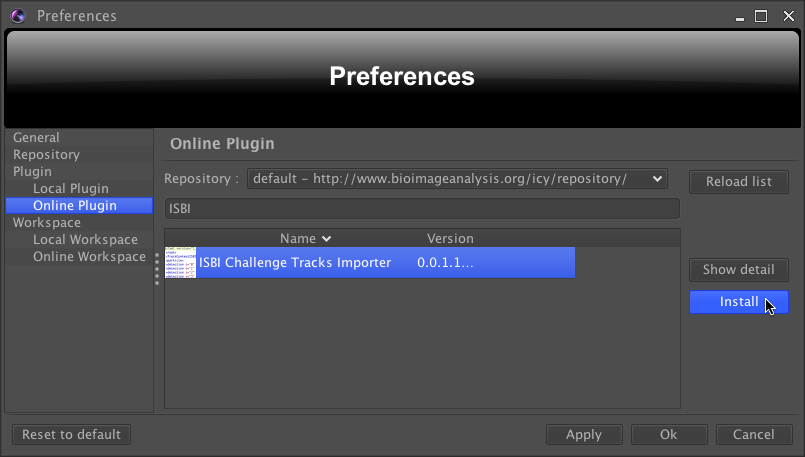
Computation of performance evaluation measures is also implemented as a plugin for Icy named Tracking Performance Measures. Installation of plugins in Icy is made easy by the existence of an official plugin repository that is accessible through the Icy user interface. The following steps will install the plugin:

1. Open the plugin repository explorer by clicking on the tab Plugins and then selecting online plugin in the Setup box.

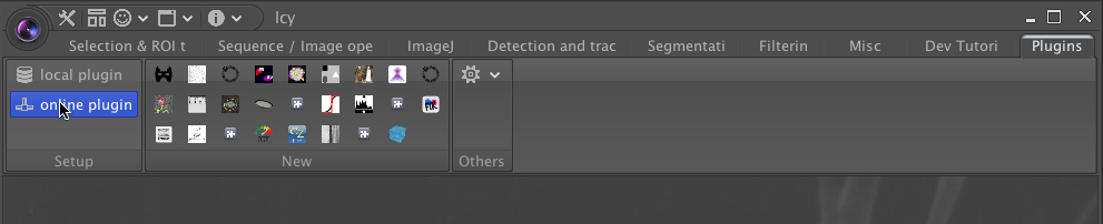
2. Select the Online plugin item in the tree in the left panel and type Tracking Performance in the search box. The Tracking Measure Performance plugin should appear in the list of available plugins.

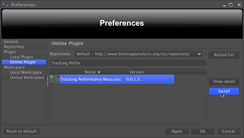
3. Click on the button Install to download and install the plugin.

The Tracking Measure Performance plugin is a special type of application that needs the plugin Track Manager to run. This plugin provides many useful tools for track visualization and track processing. It should have already been automatically installed.

In order to load tracks to the Track Manager plugin from an XML file that follows the format of the challenge, it is required to install a plugin to parse the file. This plugin is named ISBI Challenge Tracks Importer. To install it, one should proceed with the same steps as for the installation of the Tracking Performance Measures plugin, but the keyword ISBI has to be searched for instead.

In the tab Detection and Tracking, selecting Track Manager yields the interface of the Track Manager plugin to be displayed.

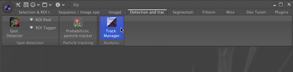
One should then click on the Add Track Processor button and select ISBI Challenge Tracks Importer.

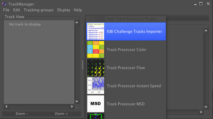
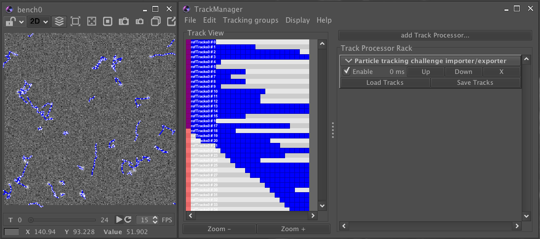
The interface of the plugin should then be displayed inside the Track Manager. In order to load a tracks from a XML file, one has to click on Load Tracks, choose a valid name for the group of tracks, and select the file.

Opening an image sequence with Icy automatically results in overlaying the tracks that have been loaded in the Track Manager to the image sequence.

To compute tracking performance, one has first to launch the Track Manager plugin and import track files. Then, the Tracking Performance Measures plugin can be run by clicking on the Add Track Processor button in the Track Manager interface and selecting the plugin in the list of track processors.

The performance computation requires the user to select the groups of tracks to be compared in the Track groups selection box. In the Track Pairing box, the distance field is the gate ε used for measuring distances between positions, as described above.

Once the Pair tracks button is clicked, the optimal pairing is computed and the tracking performance measures are automatically displayed in the box Tracking performance. The results can be exported to a text file by clicking Save results.

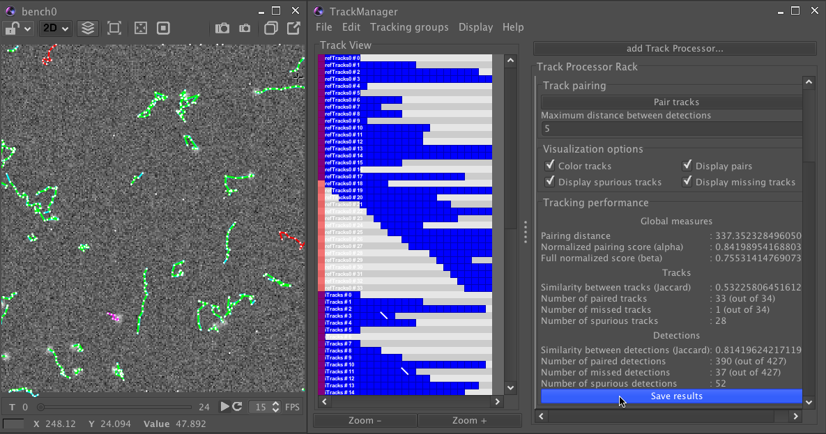
If tracks are overlaid to an image sequence, a color coding is used for tracks depending on their pairing status:

• Reference tracks that are paired to a non-dummy track are displayed in cyan.
• Candidate tracks that are paired to a reference track are displayed in green.
• A thin yellow line links detections that are paired.
• Reference tracks that are paired to a dummy track (FN tracks) are displayed in magenta.
• Candidate tracks that are not paired (FP tracks) are displayed in red.

• Training image data and ground truth for virus scenario
• Training image data and ground truth for vesicle scenario
• Training image data and ground truth for receptor scenario
• Training image data and ground truth for microtubule scenario
• Technical note describing performance measures
• Stand-alone application for performance computation
• Track file converter for the MTrackJ plugin
• Challenge image data for virus scenario
• Challenge image data for vesicle scenario
• Challenge image data for receptor scenario
• Challenge image data for microtubule scenario

Edited Feb. 11, 2012 by the Particle Tracking Challenge Committee